What Is Decision Tree Learning In Machine Learning?

Welcome, eager reader! Let’s start off with a quick dive into the world of Machine Learning. It’s a subfield of Artificial Intelligence where we teach computers to learn and make decisions from data. It’s like teaching a toddler to identify objects, but instead, we’re teaching machines. In this realm, Decision Tree Learning plays a prominent role. Here’s why…

Importance and Role of Decision Trees in Machine Learning

Surely, you’ve heard of Decision Trees. These guys are big shots in Machine Learning! Why so? Well, they can sort through vast amounts of data, detecting patterns that may not be readily apparent. They help machines mimic the human decision-making process, almost like a visual flowchart for machines! They play a crucial role in both supervised and unsupervised learning; how cool is that?

Understanding Decision Trees

So, what on earth is a Decision Tree? Simply put, it’s a flowchart-like model that helps make decisions. Picture a tree! It begins at the root (decision point), then splits into branches (possible outcomes), leading to leaves (final results). In terms of Machine Learning, Decision Trees are algorithms that train models to classify data or predict outcomes. They are direct, intuitive, and visualize the process in a way that’s pretty easy to grasp.

What is a Decision Tree?

A Decision Tree is a fantastical beast in the machine learning universe. Think of it as a guide to making decisions, somewhat like a flowchart. At its core, a decision tree uses a tree-like graph or model to predict possible outcomes. It sorts through data and makes classifications or regression decisions. So, akin to a marvelous guide deciding your fate, a decision tree weighs options and makes educated choices.

How Does a Decision Tree Work?

Decision Trees mimic the human thinking process. When posed a problem, each internal node in the decision tree checks a condition and takes a decision to move further depending upon the condition’s outcome. It uses the If-Then logic. To reach a decision or prediction, each path from the root node (start) to a leaf node (end) forms a decision rule. It’s like playing a strategic, rule-based board game!

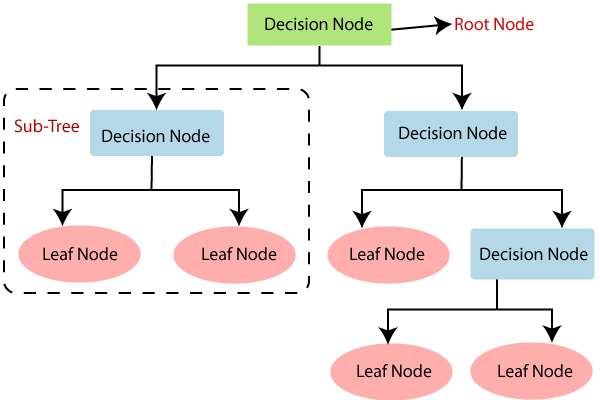
Components of a Decision Tree

A Decision Tree is made up of three key components:

Root Node: A node with no incoming edge. It embodies the entire sample and this further gets divided into two or more homogeneous sets.
Branches: These indicate outcome of a test and connect to the next node or Leaf.
Leaf Nodes: Terminal nodes representing outcomes, also known as ‘Decision’. These are the goals, the answers to your queries.

Root Node

Imagine you’re navigating a new city. The first decision you make? Perhaps to go left or right at the crossroads from your starting point. In the world of Decision Trees, this initial point is called the Root Node. It’s the very first choice that influences all the following decisions. Think of it as the inception of your tree, where all the branches initially sprout from.

The Branches of a Decision Tree

In a decision tree, think of branches as paths from the root (or another internal node) to a decision — they symbolize the choices you make. Each branch connects two nodes and represents a possible outcome for a given test. So, essentially, your decisions, or the steps you take towards the final decision, are dictated by these branches. They take the myriad possibilities and reduce them to a clear path forward.

Leaf Nodes

Let’s look at the ultimate decision-makers in this process — the Leaf Nodes. These are the end points or the ‘leaves’ of a decision tree. They don’t contain any further branches, and they ultimately determine the outcome of the decision. All paths in a decision tree will eventually lead to a leaf node. It’s like reaching the end of a choose-your-own-adventure book – you’ve made your choices and now you see the result.

Types of Decision Trees

In the realm of Machine Learning, we primarily encounter two distinct types of decision trees.

Categorical Variable Decision Tree: This type is best-suited when our target variable (or the decision) is categorical.
Continuous Variable Decision Tree: Conversely, when our decision outcome is a continuous number, we lean towards this type.

Though different, they both offer fantastic avenues for making sense of complex data.

Categorical Variable Decision Tree

A Categorical Variable Decision Tree plays with categorical, yes/no-type data. For instance, whether someone will enjoy a book. Factors might include:

Is it their preferred genre?
Does it feature their favorite character type?
Is the book by an author they like?

Each answer branches off, guiding to the final verdict. These trees are invaluable for prediction in datasets with categorical variables.

Continuous Variable Decision Tree

Continuous variable decision trees are a bit more intricate than their categorical counterparts. They excel at handling real numbers or numerical data. For instance, let’s say we’re predicting house prices. The decision tree will make splits based on questions like, is the house price more or less than $800,000? thereby, offering valuable insight and assisting in accurate predictions. Not so tough, right?

In our next section, we’ll dive deeper into Decision Tree Learning!

Process of Decision Tree Learning

In machine learning, the Decision Tree Learning follows steps similar to human decision-making process. It’s all about asking the right questions!

We begin with the entire data at the root
Split the data based on certain conditions
Repeat the process until a clear decision can be made

This learning process uses specific algorithms such as ID3, C4.5 or CART. It’s simple, but incredibly effective!

Key Concepts in Decision Tree Algorithms

We can’t talk about these algorithms without mentioning concepts like entropy and information gain.

Entropy: Measuring Uncertainty

Entropy, originating from thermodynamics as a measure of molecular disorder, is used in Decision Tree Learning to gauge randomness or uncertainty in data points. If entropy is 0, it indicates a completely homogeneous (no uncertainty) dataset, while an entropy of 1 suggests a perfectly diverse (high uncertainty) dataset. Thus, in the context of decision trees, Entropy helps to decide which feature splitting will best simplify our tree.

Information Gain

In Decision Tree Learning, Information Gain plays a pivotal role. It’s a statistical property that gauges how well a particular attribute separates the training examples based on their target classification. Put simply, it’s all about reducing uncertainty!

The attribute with the highest information gain is usually chosen as the starting point for a decision tree. This makes information gain key to forming intelligent, well-structured decision trees!

Advantages of Decision Tree Learning

Embracing Decision Tree Learning opens up a multitude of benefits. Here’s why it’s a hot pick:

Interpretability: They are easy to understand and interpret, making them incredibly user-friendly.
Data Preparation: Decision Trees require little data preparation.
Handling Nonlinear Relationships: They effectively capture nonlinear relationships between features and the target.
Flexibility: They can handle both categorical and numerical data.

In a nutshell, their simplicity and flexibility make Decision Trees a key tool in Machine Learning.

Limitations of Decision Tree Learning

While decision trees are an immensely useful tool in machine learning, they do come with their fair share of limitations.

Perhaps the most significant is their tendency to overfit. Decision trees can create complex structures that perfectly fit the training data but perform poorly on new, unseen data.
Additionally, they can be sensitive to small changes in data. Simply changing a few data points can lead to a completely different tree structure.
Decision trees also struggle to express XOR, parity or multiplexer problems.

Decision Tree Learning in Real-life Applications

In reality, decision tree learning is ubiquitously put to use. Some examples include:

Healthcare: It aids doctors in diagnosing diseases by analyzing patient history.
Business Strategy: Companies utilize it to predict consumer behavior, which directly influences their strategies.
Risk Management: Decision trees facilitate understanding of possible outcomes, helping to mitigate risks.
Quality Control: It helps in predicting the potential flaws in products, earmarking areas for improvement.

Decision Tree Learning with Python

Steps to Building a Decision Tree:

Select the best attribute: Choose the attribute that provides the best split, i.e., the one that best differentiates the data into classes. Various criteria like Gini impurity or information gain can be used for this.
Split the Dataset: Based on the chosen attribute’s value, divide the dataset into subsets.
Repeat: Continue this process recursively for each subset until one of the stopping conditions is met, such as the dataset being split perfectly or reaching a predefined tree depth.

Hands-on with Python

Let’s build a simple decision tree using Python’s scikit-learn library:

# Import necessary libraries
from sklearn.datasets import load_iris
from sklearn.model_selection import train_test_split
from sklearn.tree import DecisionTreeClassifier
from sklearn import tree
import matplotlib.pyplot as plt

# Load the Iris dataset
iris = load_iris()
X = iris.data
y = iris.target

# Split the data into training and testing sets
X_train, X_test, y_train, y_test = train_test_split(X, y, test_size=0.2, random_state=42)

# Create a decision tree classifier instance and train it
clf = DecisionTreeClassifier(criterion='entropy', max_depth=3)
clf.fit(X_train, y_train)

# Measure accuracy on the test set
accuracy = clf.score(X_test, y_test)
print(f"Test Accuracy: {accuracy:.4f}")

# Visualize the trained decision tree
fig, ax = plt.subplots(figsize=(12, 12))
tree.plot_tree(clf, filled=True, feature_names=iris.feature_names, class_names=iris.target_names, rounded=True)
plt.show()

Understanding the code

We’ve imported the necessary modules and loaded the Iris dataset, a popular dataset in machine learning. It contains 3 classes of 50 instances each, where each class refers to a type of iris plant.
We split the data into a training set (80%) and a test set (20%).
We created a DecisionTreeClassifier object, specifying the criterion as ‘entropy’ (a measure of information gain) and set the maximum depth of the tree to 3. You can experiment with other parameters like criterion='gini' for Gini impurity.
After training the classifier, we measured its accuracy on the test set.
Finally, we visualized the decision tree, which can provide valuable insights into the decision-making process.

Conclusion

Let’s take a quick rewind. We started by unpacking decision trees in machine learning, dug into the key components, types, and intricacies of how decision trees learn. We explored the concepts underpinning tree algorithms, and their pros and cons, before peeking at exciting real-world applications. As we bid adieu, remember, decision tree learning is a powerful tool, but like other ML techniques, it’s about finding the right fit for the problem at hand.